Page 7 - Fister jr., Iztok, and Andrej Brodnik (eds.). StuCoSReC. Proceedings of the 2017 4th Student Computer Science Research Conference. Koper: University of Primorska Press, 2017
P. 7
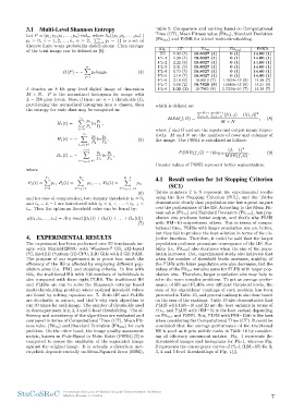
Multi-Level Shannon Entropy Table 2: Comparison and ranking based on Computational
Time (CT), Mean Fitness value (Fitm), Standard Deviation
Let P = (p1, p2, p3, . . . , pn) inδn, where δn{(p1, p2, . . . , pn) | (Fitstd) and PSNR for 2-level multi-thresholding.
n
pi ≥ 0, i = 1, 2, . . . , n, n ≥ 2, i=1 pi = 1} is a set of
discrete finite n-ary probability distributions. Then entropy Alg. CT Fitm Fitstd PSNR
18.8027 (1) 0 (1)
of the total image can be defined as [9]: HS 1.92 (5) 18.8027 (1) 0 (1) 14.60 (1)
PL-1 1.90 (4) 18.8027 (1) 0 (1) 14.60 (1)
n (4) PL-2 2.22 (8) 18.8027 (1) 0 (1) 14.60 (1)
PL-3 2.31 (9) 18.8027 (1) 0 (1) 14.60 (1)
H(P ) = − pilog2pi PL-4 1.73 (3) 18.8027 (1) 0 (1) 14.60 (1)
PL-5 2.14 (7) 18.8010 (7) 1.1024e-13 (9) 14.60 (1)
i=1 PL-6 2.10 (6) 18.7820 (9) 1.0669e-13 (8) 14.38 (7)
PL-7 1.68 (2) 18.7985 (8) 5.3334e-16 (7) 14.31 (9)
I denotes an 8 bit gray level digital image of dimension PL-8 1.02 (1) 14.38 (7)
M × N . P is the normalized histogram for image with
L = 256 gray levels. Now, if there are n − 1 thresholds (t), which is defined as: N −1 jM=−01[f (i, j) − G(i, j)]2 ,
partitioning the normalized histogram into n classes, then M SE(f, G) = i=0 M ×N
the entropy for each class may be computed as:
t1 pi ln pi , (8)
i=0 P1 P1
H1(t) = −
H2(t) = − t2 pi ln pi , (5) where f and G and are the inputs and output image respec-
i=t1 +1 P2 P2 tively. M and N are the numbers of rows and columns of
the image. The PSNR is calculated as follows:
Hn(t) = − L−1 pi ln pi , (L − 1)2 (9)
i=tn−1 +1 Pn Pn P SN R(f, G) = 10log10 M SE(f, G) .
Greater values of PSNR represent better segmentation.
where
t1 t2 L−1 4.1 Result section for 1st Stopping Criterion
P1(t) = pi, P2(t) = pi, . . . , Pn(t) = pi, (SC1)
i=0 i=t1 +1 i=tn−1 +1 Tables numbers 2 to 5 represent the experimental results
using the first Stopping Criterion (SC1), and the Tables
(6) demonstrate clearly that population size has a great impact
over the performance of the HS. According to the Mean Fit-
and for ease of computation, two dummy thresholds t0 = 0, ness value (Fitm) and Standard Deviation (Fitstd), less pop-
and tn = L − 1 are introduced with t0 < t1 < . . . < tn−1 < ulation size produces better output, and that’s why PLHS
tn. Then the optimum threshold value can be found by: with HM=10 outperforms others. But in terms of compu-
tational time, PLHSs with larger population size are better,
ϕ(t1, t2, . . . , tn) = Arg max([H1(t) + H2(t) + . . . + Hn(t)]) but they fail to produce the best solution in terms of the ob-
(7) jective function. Therefore, it could be said that the larger
population performs premature convergence of the HS. Sta-
4. EXPERIMENTAL RESULTS bility (i.e. Fitstd) also decreases when the size of the popu-
lation increases. But, experimental study also indicates that
The experiment has been performed over 50 benchmark im- when the number of threshold levels increases, stability of
ages with MatlabR2009b with Windows-7 OS, x32-based the PLHS with lower population size also decreases, but the
PC, Intel(R) Pentium (R)-CPU, 2.20 GHz with 2 GB RAM. values of the Fitstd remains same for PLHS with larger pop-
The purpose of our experiment is to prove how much the ulation size. Therefore, larger population size may help to
efficiency of the HS is affected by employing different pop- solve the more complex problems. To get an average perfor-
ulation sizes (i.e. HM) and stopping criteria. In line with mance of HS and PLHSs over different threshold levels, the
this, the traditional HA with 100 numbers of individuals is sum of the algorithms’ rankings of each problem has been
also compared with these eight PLHS. The traditional HS presented in Table 10, and general ranking is also done based
and PLHSs are run to solve the Shannon’s entropy based on the sum of the rankings. Table 10 also demonstrates that
multi-thresholding problem where optimal threshold values PLHS with HM=10 and 20 are the best variants in terms of
are found by solving equation no. 7. Both HS and PLHSs Fitm and PLHS with HM=10 is the best variant depending
are stochastic in nature, and that’s why each algorithm is on Fitstd and PSNR. But, PLHS with HM=1280 is the best
run 30 times for each image. The number of thresholds used when considering the Computational Time (CT). It could be
in this experiment is 2, 3, 4 and 5-level thresholding. The ef- concluded that the average performance of the traditional
ficiency and consistency of the algorithms are evaluated and HS is good as it gets middle ranks in Table 10 by consider-
compared in terms of Computational Time (CT), Mean Fit- ing all efficiency assessment metrics. Fig. 1 represents the
ness value (Fitm) and Standard Deviation (Fitstd) for each thresholded images and histograms for PL-1, whereas Fig.
problem. On the other hand, the image quality assessment 2 represents the convergence curves of PL-1 (HM=10) for 2,
metric, known as Peak-Signal to Noise Ratio (PSNR) [2] is 3, 4 and 5 level thresholdings of Fig. 1(j).
computed to assess the similarity of the segmented image
against the original image. It is actually a distortion met-
ric,which depends crucially on Mean-Squared Error (MSE),
StuCoSReC Proceedings of the 2017 4th Student Computer Science Research Conference 7
Maribor, Slovenia, 11 October